Power BI DAX to Sigma formulas: a practical cheat sheet

Power BI's DAX SUM and AVERAGE have straightforward Sigma counterparts: Sum and Avg. More complex measures need their calculation context rebuilt. In particular, CALCULATE isn't simply another spelling of SumIf, and DAX DISTINCTCOUNT counts a BLANK value that Sigma's CountDistinct excludes when represented as null.

Use this guide for calculation translation. Our Power BI-to-Sigma migration plan covers the broader work of inventorying models, choosing a pilot and planning rollout.

The visual reference

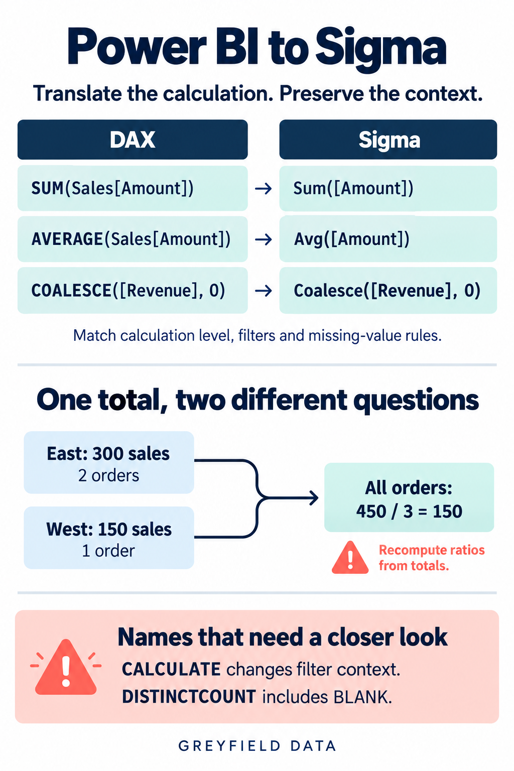
Open the full-size diagram. Copyable expressions and their assumptions follow.

A small dataset makes differences visible

Use this three-order CSV. Import the table as Sales when using the DAX examples. Each row is one order; Amount and Cost are numeric. Treat the missing Customer value as a DAX BLANK or Sigma null for the distinct-count example, and confirm your import actually does that.

Order	Region	Amount	Cost	Customer
O1	East	100	60	C1
O2	East	200	140	C1
O3	West	150	90	null

Revenue is 450, cost is 290 and profit is 160. East contributes 300 across two orders; West contributes 150 across one. These are locally checked arithmetic results. The product behavior below is grounded in documentation, not a claim that this example has passed live Power BI and Sigma tests.

The close matches

Task	DAX expression	Sigma expression
Revenue	SUM(Sales[Amount])	Sum([Amount])
Average order amount	AVERAGE(Sales[Amount])	Avg([Amount])
Replace missing revenue with zero	COALESCE([Revenue], 0)	Coalesce([Revenue], 0)

For the last row, [Revenue] means an already-defined measure or calculation at the intended level. The example assumes numeric revenue, and a deliberate decision to display missing revenue as zero. DAX works with BLANK; Sigma's Coalesce selects the first non-null argument. DAX COALESCE, Sigma Coalesce

A Power BI measure is evaluated in its reporting context. In Sigma, choose the row, group or summary level explicitly. Use a Region grouping for East 300 and West 150, or a table summary for 450. The function name alone doesn't establish that level. DAX overview, Sigma tables

The numeric functions are documented in DAX SUM, DAX AVERAGE, Sigma Sum and Sigma Avg.

SUMX: preserve the row expression

This DAX measure calculates profit on each order and adds it:

Profit = SUMX(Sales, Sales[Amount] - Sales[Cost])

For this flat, numeric sample, create a row-level Sigma column called Profit:

[Amount] - [Cost]

Then aggregate it at the intended group or summary level:

Sum([Profit])

The row profits are 40, 60 and 60; total profit is 160. Inspect the three row results before inspecting the total. This two-step translation applies to this expression over this table. A SUMX over a filtered or constructed table needs that input population preserved too. DAX SUMX

Set up row calculations, grouped results and summaries

Load the three-order CSV into a table element, with Amount and Cost numeric and Order, Region and Customer as text. Confirm that the blank Customer on O3 becomes null for the stated count example.

Add the Profit row column from the SUMX section. Under Groupings, add Region; under that group's Calculations, add Sum([Amount]) and Sum([Profit]). Expected regional pairs are East revenue 300/profit 100 and West revenue 150/profit 60. Then use Show summaries → Add summary → New summary to calculate whole-table revenue 450 and profit 160. Sigma grouping and summaries

Keep the source row count visible during the rebuild. These formulas assume order grain. If joining products or order lines changes three orders into more rows, fix that population before trusting a revenue measure. A distinct order count can remain three even while duplicated Amount values inflate revenue.

CALCULATE: a matching total can hide a different rule

Consider this DAX measure:

East Revenue =
CALCULATE(SUM(Sales[Amount]), Sales[Region] = "East")

With the whole sample available, this Sigma aggregate also produces 300:

SumIf([Amount], [Region] = "East")

That matching result doesn't establish general equivalence. CALCULATE can replace an existing filter on the same column. If a source selection filters Sales[Region] directly to West, the DAX filter above replaces it with East. By contrast, a Sigma SumIf operating on a source already reduced to West cannot recover East records. DAX CALCULATE, Sigma SumIf

The DAX example assumes a filter directly on this column, not a different related dimension table. Relationships can change the outcome. Record which filters a measure replaces, retains or removes, then design the target sources and controls around that requirement. Test a conflicting selection, not only the unfiltered dashboard.

Implement the intended CALCULATE behavior

There are two different requirements that can hide behind “East Revenue.” Decide which one the source measure implements before building its replacement.

Requirement A: East within the current selection. If the user selects West, no East rows should contribute. This is an intersection. In DAX, a same-column example uses KEEPFILTERS:

East Within Selection =
CALCULATE(
  SUM(Sales[Amount]),
  KEEPFILTERS(Sales[Region] = "East")
)

KEEPFILTERS retains the intersection with existing filters on that column. Microsoft KEEPFILTERS

In Sigma, target the working Sales table with the Region control and calculate SumIf([Amount], [Region] = "East") in its summary. The unfiltered and East-selected cases should contribute 300. A West selection leaves no qualifying East records. Agree whether that state displays null or zero rather than treating either display as a filter-design decision.

Requirement B: East regardless of the Region selection. This matches the earlier same-column CALCULATE replacement example. Create a separate table element named EastKPI from the source before the Region restriction. Target the normal sales view with the Region control, and leave EastKPI untargeted by that control. Apply any required period or product filters to both branches.

In EastKPI, create a summary:

SumIf([Amount], [Region] = "East")

The intended KPI remains 300 for All, East and West selections in this sample. It remains responsive to the other filters you deliberately retain. A Region-filtered common parent would invalidate this design because filters propagate downstream. Review the control's Properties → Targets and its target column, not just the label on the canvas. Sigma control targets, Filter propagation

This handles one stated measure contract. It doesn't automatically reproduce relationship-based filters, context transition or every CALCULATE modifier. If the original expression uses those features, add their cases to the acceptance record instead of treating this branch pattern as universal DAX support.

DIVIDE: define the zero-denominator result

In DAX:

Average Order Value =
DIVIDE(SUM(Sales[Amount]), DISTINCTCOUNT(Sales[Order]))

For these unique, populated Order IDs, the Sigma expression at the corresponding aggregate level is:

Sum([Amount]) / NullIf(CountDistinct([Order]), 0)

The sample returns 450 divided by 3, or 150. NullIf turns a zero count into null rather than leaving a zero divisor. DAX DIVIDE defaults to BLANK on division by zero; if the original measure specifies an alternate result, make that requirement explicit in the target and test it. DAX DIVIDE, Sigma NullIf

Recompute a total ratio from total revenue and total order count. To see why, change O3's Amount to 90 in a separate test copy. East's average remains 150, West's becomes 90, and the overall average is 390 divided by 3, or 130. Averaging the two regional averages would give 120. The published CSV remains unchanged.

Test ratios with deliberately uneven groups

The original sample has average order value 150 in both regions, so it won't expose an average-of-averages error. Use the ratio test CSV, which changes only O3's Amount to 90.

Population	Revenue	Distinct orders	Average order value
East	300	2	150
West	90	1	90
All	390	3	130

Keep the summary expression as revenue divided by distinct orders. If the grand total is 120, it averaged the two displayed regional averages. If it is 240, it added them. Neither result represents average order value across the three orders.

For margin, the same principle applies: this variant has total profit 100 and revenue 390, giving about 25.64%. Calculate the ratio from total profit and revenue, rather than averaging order or region margins. Keep precision in the calculation and round only the displayed percentage.

DISTINCTCOUNT: test the missing customer

For the Customer column, DAX DISTINCTCOUNT(Sales[Customer]) counts C1 and BLANK, yielding two. Sigma CountDistinct([Customer]) excludes null and empty values, yielding one under the stated import assumptions. These are different definitions, even though the function names sound equivalent. DAX DISTINCTCOUNT, Sigma CountDistinct

Decide whether the business metric is known customers or distinct values including a missing category. Don't silently label a missing identity as a known customer merely to match a number. Also test a selection with no rows; missing-result behavior is a separate case from a row containing a missing value.

Make blank-counting a deliberate metric

For a known-customer metric, CountDistinct([Customer]) returns one in the supplied sample. If the requirement is instead “distinct populated values plus one missing category when any missing records exist,” create a separate aggregate:

CountDistinct([Customer])
+ If(CountIf(IsNull([Customer])) > 0, 1, 0)

Expected result: two. This explicitly counts one missing category, rather than replacing every missing customer with a made-up customer identifier. Test the case with only C1, only the null row, and both together. Expected results are one, one and two. CountDistinct, CountIf, IsNull

Keep this narrower than a claim of complete DAX parity. The formula assumes missing values are null, not empty strings, and the input has at least one row. Define an empty-population display separately, since DAX DISTINCTCOUNT returns BLANK when there are no rows.

A small acceptance checklist

Download the shared validation checklist. It includes expected results for all three guides and blank fields for observed results, evidence and reviewer. Use the Power BI rows first, then add model-specific cases.

Before signing off, compare the same source cutoff and authorized population in both products. Check an unfiltered total, a conflicting Region selection, the null customer and the uneven-group ratio. A formula that passes only the unfiltered total hasn't demonstrated that it preserves the report's behavior.

Use our seven DAX migration tests to record totals, dates, blanks, ratios and relationships. For help with a model, bring the measure definitions and their filter requirements to a Power BI-to-Sigma assessment.