Excel to Sigma functions: a practical formula cheat sheet

Excel's SUM maps to Sigma's Sum, AVERAGE to Avg, and conditional sums such as SUMIFS to SumIf. For exact-key lookups, start with Sigma's Lookup. The bigger change is where the calculation runs: Sigma uses columns, groups and summaries rather than a selected range of spreadsheet cells.

That means a formula can be spelled correctly and still answer the wrong question. Before translating it, decide whether you need one result per row, per group, or for the whole table.

The visual cheat sheet

The graphic uses the same four rows as the examples below. The arrows show two different ways to aggregate those rows, not two steps in one calculation.

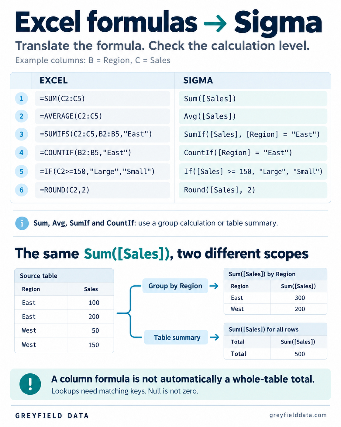
Open the full-size graphic. The formulas are also written below so you can copy them.

Start with four rows

Paste this table into Excel starting at A1, or download the example CSV. In Sigma, use a table with the same column names and numeric types for Sales and Cost.

Order	Region	Sales	Cost	SKU
O1	East	100	60	A
O2	East	200	140	A
O3	West	50	20	B
O4	West	150	90	C

Sales total 500, cost totals 310, and profit is 190. The average sale is 125. These are locally checked example values; this article doesn't claim a completed live Sigma implementation.

Build the example as a Sigma table

Start with the sales and Products files linked in this guide. Keep their key columns as text and Sales and Cost as numbers. For the lookup exercise, both elements must use the same connection. If your upload workflow places them on different connections, load them into a shared supported source before attempting the lookup.

1. Open the workbook for editing and add the sales table as a data element.
2. Add a calculated column named Profit and enter [Sales] - [Cost]. Check the four rows: 40, 60, 30 and 60.
3. Add Region under Groupings. Add Sum([Sales]) under that group's Calculations. Check East 300 and West 200.
4. Add a table summary with Sum([Profit]). It should show 190 across the four rows.

These separate checks catch different mistakes. Incorrect row profit points to source types or the expression. Correct rows with incorrect regional results point to grouping or filters. A correct regional display with an incorrect summary calls for inspecting the summary's formula and population. Sigma table setup

Six common formula translations

For the first four formulas, use a Sigma table summary to reproduce the whole-range Excel result. A grouping calculation instead evaluates the relevant group. The last two are row calculations.

SUM becomes Sum

Excel: =SUM(C2:C5)

Sigma: Sum([Sales])

Expected table-summary result: 500. Sigma's Sum documentation explains the aggregation behavior. The column reference names the data; it doesn't by itself specify a whole-table total.

AVERAGE becomes Avg

Excel: =AVERAGE(C2:C5)

Sigma: Avg([Sales])

Expected table-summary result: 125. At the Region grouping, Avg gives East 150 and West 100. Check missing values and data types when translating a real workbook; this example contains four populated numeric sales values.

SUMIFS becomes SumIf with conditions

Excel: =SUMIFS(C2:C5,B2:B5,"East")

Sigma: SumIf([Sales], [Region] = "East")

Expected table-summary result: 300. Excel SUMIFS uses range/criteria pairs. Sigma SumIf takes the value column followed by logical conditions.

For East sales above 100:

Excel:
=SUMIFS(C2:C5,B2:B5,"East",C2:C5,">100")

Sigma:
SumIf([Sales], [Region] = "East", [Sales] > 100)

The result is 200. Sigma combines those conditions with AND. Also watch Excel's singular SUMIF: its argument order differs from SUMIFS, so changing only the function name isn't enough.

COUNTIF becomes CountIf with a condition

Excel: =COUNTIF(B2:B5,"East")

Sigma: CountIf([Region] = "East")

Expected table-summary result: 2. CountIf counts rows meeting the condition in the calculation's scope. That is an order count here only because this example has one row per order. On order-line data, two qualifying lines can belong to one order.

IF becomes If

Excel: =IF(C2>=150,"Large","Small")

Sigma: If([Sales] >= 150, "Large", "Small")

Expected row results: Small, Large, Small, Large. Sigma's If can also accept multiple condition/value pairs; the first true condition wins. Put your conditions in the intended order rather than assuming every branch is evaluated.

ROUND becomes Round

Excel: =ROUND(C2,2)

Sigma: Round([Sales], 2)

The whole-number inputs stay unchanged. Round changes the numeric result; formatting controls how many decimal places readers see. Showing 100.00 doesn't require changing the underlying 100. Test midpoint and negative rounding separately if your financial model depends on those cases.

More than one condition: AND, OR and distinct orders

The earlier East-and-over-100 example uses AND and returns 200. For East or a sale above 100, use one combined logical condition:

SumIf([Sales], [Region] = "East" or [Sales] > 100)

The qualifying orders are O1, O2 and O4, totaling 450. Adding an East subtotal to an over-100 subtotal would count O2 twice and produce 650. OR means a qualifying row contributes once. SumIf conditions

For unique East orders, use:

CountDistinctIf([Order], [Region] = "East")

The result is two here. If a real table has multiple order lines, CountIf counts qualifying rows while CountDistinctIf counts qualifying distinct identifiers. Define whether an order qualifies when any line matches or only when its complete order meets a condition. Those are different metrics. CountDistinctIf

The most important difference: calculation level

An Excel range such as C2:C5 explicitly selects four cells. A Sigma aggregate is evaluated at its calculation level. In an ungrouped table's ordinary calculated column, an aggregate can evaluate per row. Putting Sum([Sales]) there isn't the same as creating a table summary.

For a regional result, follow Sigma's table grouping instructions: add Region under Groupings, then add the Sales calculation under that grouping's Calculations. Use Sum([Sales]). The example should produce East 300 and West 200.

For one overall result, select Show summaries, then Add summary and New summary, and enter Sum([Sales]). With the four example rows included, the result is 500.

This is similar to choosing the fields and aggregation in an Excel PivotTable, but don't assume the interfaces or every calculation behave identically. Our Sigma table grouping guide explains the layout side.

XLOOKUP needs a key check before Lookup

Suppose a second table named Products contains unique SKU/category pairs: A/Core and B/Add-on. C has no product match. Download the Products CSV.

Excel, with Products defined as an Excel table:

=XLOOKUP(E2,Products[SKU],Products[Category],"Unmapped")

Sigma, with a Products data element on the same connection:

Coalesce(
  Lookup([Products/Category], [SKU], [Products/SKU]),
  "Unmapped"
)

The intended results are Core, Core, Add-on and Unmapped. This example assumes the matching category values aren't null. If a matching product has a null category, the Sigma formula also labels it Unmapped; Excel's if_not_found argument applies to a missing match instead. Track match status separately when that distinction matters.

XLOOKUP normally searches from the first item and uses exact matching by default. Sigma's Lookup takes the return formula first, then local/external key pairs. It can also aggregate matching target records, so it isn't a promise to reproduce every XLOOKUP mode.

Validate unique product keys for this scalar example, review unmatched keys, and keep the source table's row count and sales total intact. For multipacks and reused identifiers, see SKU mapping without breaking margin.

Make lookup failures visible

Create two intermediate columns before applying a friendly label:

Matched SKU:
Lookup([Products/SKU], [SKU], [Products/SKU])

Category:
Lookup([Products/Category], [SKU], [Products/SKU])

Then create a status column:

If(
  IsNull([Matched SKU]), "No product match",
  IsNull([Category]), "Matched, missing category",
  "Matched"
)

The supplied files should produce Matched for O1 through O3 and No product match for O4. This assumes the target SKU is unique and non-null. In a separate test copy, clear B's Category to null: O3 should now say Matched, missing category. An empty string is a separate value, so confirm how the import represents the cleared cell. Lookup, IsNull

Before using a real Products table, group it by SKU and count its rows. Investigate any key with more than one row rather than arbitrarily choosing one. After enrichment, check that the sales table still has four rows and total sales of 500. Matching a grand total doesn't establish that every order has the right category; inspect O3 and O4 individually.

Null handling isn't general error handling

Coalesce selects the first non-null argument, and its arguments need compatible types. It isn't a general substitute for every use of Excel's IFERROR. An empty string and a null also aren't automatically the same thing.

Use zero only when the business definition says a missing value means zero. Missing product cost should stay visible as missing, not become a 100% margin result. Likewise, don't assume Sigma Count means Excel's numeric-only COUNT: Sigma counts non-null, non-empty column values, or rows when called without a field.

Translate monthly date logic without turning dates into text

Download the dated sales example. It preserves the same orders and amounts and adds Order Date in column F: O1 on January 15, O2 on January 31, O3 on February 1, and O4 on February 10, 2026. Parse these as dates, not text. Use consistent business-date and time-zone settings; the expected calendar buckets below assume the displayed dates remain those four dates.

In Excel, a month-start key for F2 can be:

=DATE(YEAR(F2),MONTH(F2),1)

In Sigma:

DateTrunc("month", [Order Date])

Group by that month-start column and sum Sales. January should be 300 and February 200. DateTrunc produces a date value; a display label such as Jan 2026 should not replace the underlying date key used for sorting. With timestamps, settle the business time zone before truncating. Sigma DateTrunc, Excel DATE

For a January conditional total in Excel, use an inclusive start and exclusive next-month boundary:

=SUMIFS(C2:C5,F2:F5,">="&DATE(2026,1,1),F2:F5,"<"&DATE(2026,2,1))

In Sigma, with the date values and boundaries interpreted consistently:

SumIf(
  [Sales],
  [Order Date] >= Date("2026-01-01"),
  [Order Date] < Date("2026-02-01")
)

Expected result: 300. Check O2 and O3 on opposite sides of the boundary. For a timestamp source, a cutoff at the start of the next month avoids excluding later hours of the final day. Sigma's Date function expects ISO or Unix-formatted inputs; other text formats require explicit parsing. Sigma Date

Troubleshoot the result before adding more formulas

Symptom	Check first	Small test
Every row shows its own amount instead of 500	Calculation level	Move the aggregate to a table summary
Conditional total is 650 instead of 450	Overlapping criteria added separately	Use one OR condition and inspect O2
Unmatched and incomplete products look identical	Coalesce masks both null cases	Keep Matched SKU and Category separate
January contains O3	Date type, time zone and upper boundary	Inspect the February 1 order
A count grows after loading order lines	Rows versus unique orders	Compare CountIf and CountDistinctIf

Before moving a real report, test a normal row, an unmatched lookup, a null value and each intended grouping. Compare the same rows and filters. If you're translating a whole reporting workflow rather than a few formulas, Sigma consulting covers the modeling and validation work behind it.

Coming from another BI tool? Use the Tableau-to-Sigma functions guide or Power BI DAX-to-Sigma guide for their calculation and context differences.

Download the validation checklist to record expected and observed results, filters, data cutoff and review evidence for these examples.